Automated Exercise Assistant
Andrew Luyt 2023-06-18

Purpose
To build a machine learning model that can accurately detect if a human is performing an exercise using the incorrect form. The model will only use measurements from accelerometers on the body & dumbbell while performing dumbbell bicep curls.
This project aims to improve upon the results of a 2013 experiment yielding a model with 78.5% accuracy.
The model should be able to detect and distinguish between mistakes such as incorrect elbow position or only partially lifting the dumbbell. It should also be, at least theoretically, implementable on a wearable device such as a smart watch or FitBit.
If a person’s errors in exercise form could be detected automatically and in real-time, one possible application would be a wearable device sending an audio notification to tell the user their form is suspect: e.g. throwing elbows to the front or thrusting their hips forward.
Summary of Results
Finding that the data were not well-suited to the assumptions of Linear Discriminant Analysis, we were able to build random forest and boosted models with predictive accuracy of 99.3%.
The dataset
19623 observations over 160 variables, mostly numeric features extracted from accelerometer data streams.
The classe variable is our target. It holds five classes corresponding
to correct & incorrect form while doing the exercise:
- A: correct form
- B-E: incorrect form (common mistakes)
- B: throwing the elbows to the front
- C: lifting the dumbbell only halfway
- D: lowering the dumbbell only halfway
- E: throwing the hips to the front
Variable selection will be an important part of this problem.
These data come from a 2013 experiment, Qualitative Activity Recognition of Weight Lifting Exercises by Velloso, E.; Bulling, A.; Gellersen, H.; Ugulino, W.; Fuks, H., and was released under a Creative Commons licence. [See References for URLs]
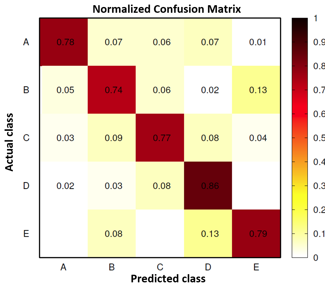
Benchmarks
The original researchers obtained 78.5% overall accuracy on this dataset, with class-specific accuracies between 74% and 86%.
Cleaning and preprocessing
Using skimr::skim() we find that 100 variables have over 97% of their
data missing. We’ll simply remove these variables. This greatly
simplifies the problem of variable selection as we now only have 59
predictors available.
classe needs to be converted to factors.
cvtd_timestamp is the time the user performed the exercise during the
original experiment and will have no bearing on future prediction so
it will be removed. user_name will be removed as well as we can’t
expect it to be available in the future.
raw_timestamp_part_1 is suspicious. In the plot below we can
distinguish the blocks of time where each classe was performed by each
subject. This appears to be due simply to the way the original
experiment was conducted: each subject was asked to perform exercises
with a given form one after another, and these times simply reflect that
sequence. When an algorithm is applied to future data (for example a
person doing their workout tomorrow) these time patterns will be
completely different, rendering this feature useless. We will remove
this variable along with raw_timestamp_part_2, and new_window for
similar reasons.

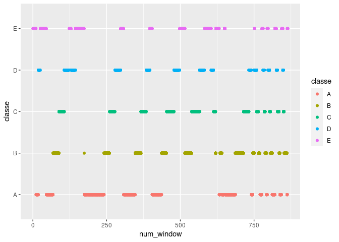
num_window has similar problems. Below, if for example num_window is
about 250, the classe will be B. This variable seems to be a
sequence identifier for blocks of information sequentially extracted
from the accelerometer data stream during feature extraction. There’s no
reason to suspect this pattern would continue in any future data. This
variable will also be removed.
Check variables for normality
Some models, like LDA, assume normal distributions of variables - how good of an assumption would this be? Using a Shapiro Test, we find that no variable is drawn from a normal distribution.
Check for near-zero-variance predictors
After removing variables full of NAs, caret::nearZeroVar() was used.
All variables have sufficient variance to be useful, in theory.
Modeling
We’ll explore a Linear Discriminant model first as a baseline and then two ensemble models generally considered to give excellent performance on classification problems: boosted trees and random forests.
Linear Discriminant Model
Earlier we found that the variables are not normally distributed, so we can’t expect good classification performance from LDA.
classe was fit to all variables and the resulting accuracy estimate
via a .632 bootstrap was 70%. The original researchers obtained 78.5%
using a different model, so we will have to improve on this.
##   Accuracy Kappa
## 1    0.703 0.624
Stochastic Gradient Boosting
Tree-based ensembles are traditionally strong performers on
classification tasks. Our first ensemble will use gradient boosting via
the gbm model.
A tuning grid is used to estimate optimal hyperparameters and
generalization error is estimated with a .632 bootstrap using caret.
##  Accuracy     Kappa
## 0.9938957 0.9922679
These are superb results compared to our baseline, perhaps too good. We’ll investigate the possibility of overfitting in the next section. The parameters of the best model found were as follows:
| n.trees | interaction.depth | shrinkage | n.minobsinnode |
|---|---|---|---|
| 450 | 6 | 0.1 | 10 |
Use an explicit train/validate set
The bootstrap results were suspiciously good and we should suspect overfitting even though boosted models overfit slowly. Checking our results by using the best model parameters we found, re-training on a randomly selected training set and checking accuracy with an independent validation set we obtain these results:
##  Accuracy     Kappa
## 0.9926983 0.9907628
| Prediction | Sensitivity | Specificity | balanced.accuracy |
|---|---|---|---|
| Class: A | 0.9982079 | 0.9966785 | 0.9974432 |
| Class: B | 0.9842105 | 0.9985260 | 0.9913683 |
| Class: C | 0.9941577 | 0.9969148 | 0.9955363 |
| Class: D | 0.9906736 | 0.9987815 | 0.9947275 |
| Class: E | 0.9935365 | 0.9997919 | 0.9966642 |
The test performance, 99.27%, is very close to the .632 bootstrap estimate. We can conclude that the model is finding a true predictive structure in the data.
Let’s also examine the top six most important variables for the boosted model:
| Overall | |
|---|---|
| roll_belt | 3117.3068 |
| pitch_forearm | 1727.4100 |
| yaw_belt | 1680.7166 |
| magnet_dumbbell_z | 1313.3487 |
| magnet_dumbbell_y | 1075.1768 |
| pitch_belt | 973.0235 |
Random Forest
The first step is to obtain a good estimate for mtry, the number of
variables to consider at each split of a tree. This is the only tuning
parameter we’ll consider, and we’ll use specialized method
randomForest::tuneRF to get a good estimate.
##
## Call:
##  randomForest(x = x, y = y, mtry = res[which.min(res[, 2]), 1])
##                Type of random forest: classification
##                      Number of trees: 500
## No. of variables tried at each split: 10
##
##         OOB estimate of  error rate: 0.57%
## Confusion matrix:
##      A    B    C    D    E class.error
## A 3901    4    0    0    1 0.001280082
## B   15 2634    8    0    0 0.008656379
## C    0   10 2380    5    0 0.006263048
## D    0    0   22 2226    3 0.011106175
## E    0    0    3    7 2514 0.003961965
Results suggest the optimal value for mtry is around 10. Literature
suggests a value for mtry around
$\sqrt{\text{number of features}} = \sqrt{55} \approx 7$ which is close.
We’ll use 10 in our model. Fitting a model with mtry=10 on the same
training set we used with the boosting method, we get these results:
##  Accuracy     Kappa
## 0.9930379 0.9911930
| Prediction | Sensitivity | Specificity | balanced.accuracy |
|---|---|---|---|
| Class: A | 0.9982079 | 0.9976275 | 0.9979177 |
| Class: B | 0.9877193 | 0.9983154 | 0.9930174 |
| Class: C | 0.9941577 | 0.9965035 | 0.9953306 |
| Class: D | 0.9875648 | 0.9991877 | 0.9933762 |
| Class: E | 0.9944598 | 0.9995839 | 0.9970218 |
The random forest obtains 99.3% accuracy on the validation set, compared to 99.26% for the boosted model. Their class-specific sensitivity, specificity, etc are also near-equal. The models are essentially equivalent in their predictive ability, though the random forest was much faster to train.
Using the generic importance function to list variable importance, the
top six variables for the random forest are the same the boosted model,
suggesting both models are finding similar structures in the data, which
increases our confidence in their correctness.
| variable | MeanDecreaseGini |
|---|---|
| roll_belt | 1008.7102 |
| yaw_belt | 658.8992 |
| pitch_forearm | 629.6978 |
| magnet_dumbbell_z | 573.8069 |
| pitch_belt | 520.7653 |
| magnet_dumbbell_y | 508.8364 |
Predictions
A test dataset of 20 observations has been provided. We’ll predict using our boosted and random forest models and compare them to each other.
pred.gbm.tt <- predict(fit.gbm.tt, df.test)
pred.rf <- predict(fit.rf, df.test)
table(pred.gbm.tt == pred.rf)
##
## TRUE
##   20
Both models predict the same values for the test set.
Conclusions
After reducing the number of variables from 160 to 52, we were able to build both random forest and boosted models with an accuracy of 99.3%, equivalent to be one false detection in 143 repetitions of a bicep curl. It seems likely that a combination of smart devices and machine learning are genuinely able to detect correct vs incorrect exercise form.
To create a real-world product there would be much more work to do, starting with creating a much larger dataset including all the other types of exercise the smart device would support - this dataset only contains observations of one exercise. Other complications such as expert consultation with exercise physiologists and liability issues would have to be taken into account, so this is where I will end this project.
References
Original Dataset:
Velloso, E.; Bulling, A.; Gellersen, H.; Ugulino, W.; Fuks, H. Qualitative Activity Recognition of Weight Lifting Exercises. Proceedings of 4th International Conference in Cooperation with SIGCHI (Augmented Human ’13) . Stuttgart, Germany: ACM SIGCHI, 2013.
Obtained from https://web.archive.org/web/20150207080848/http://groupware.les.inf.puc-rio.br/har